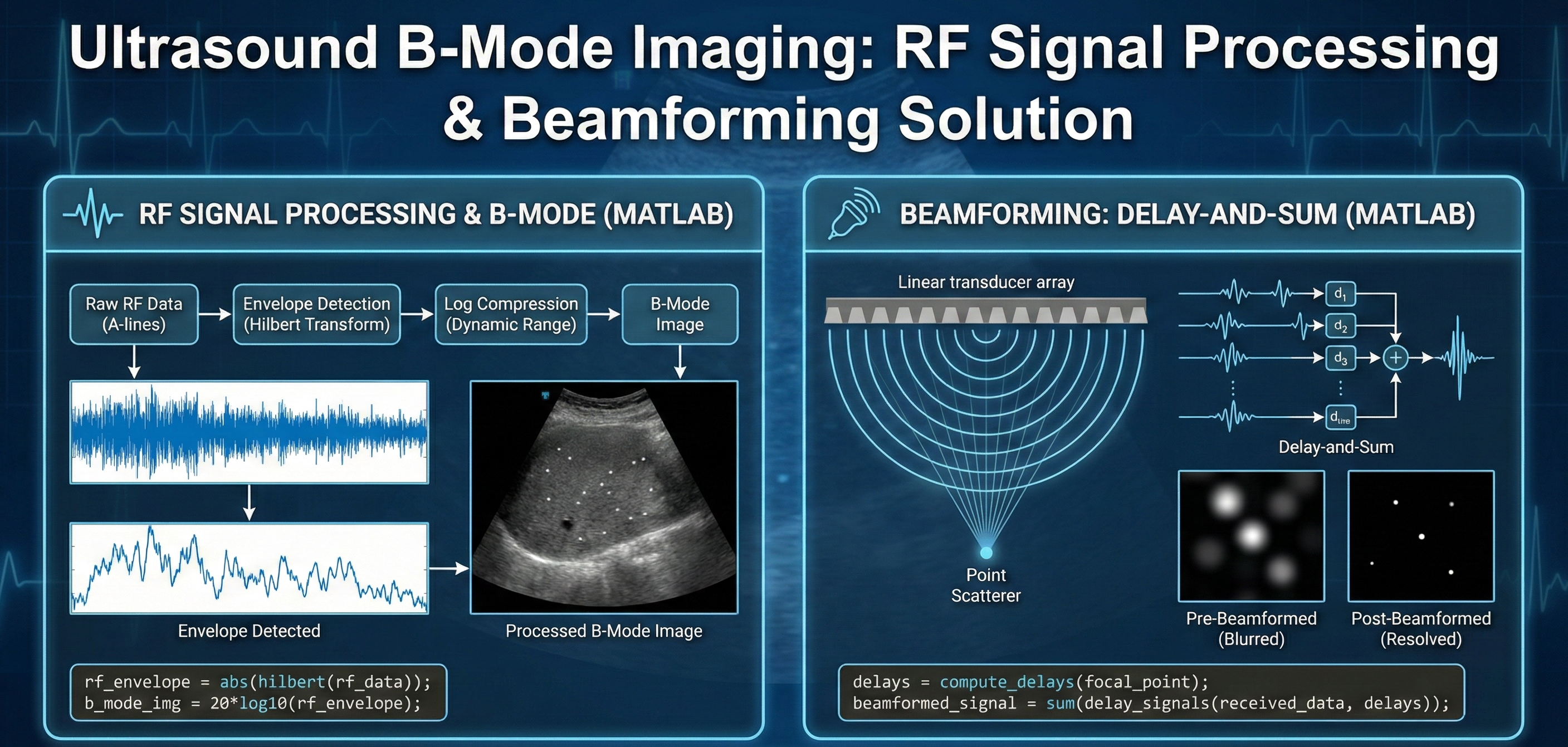
A detailed solution for processing raw ultrasound RF data into clear B-mode images using MATLAB. This download covers envelope detection (Hilbert transform), log compression, and the implementation of Delay-and-Sum beamforming to resolve point scatterers and remove image blurring.
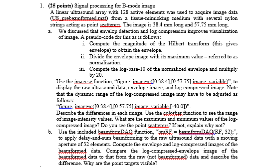
1. Signal processing for B-mode image
A linear ultrasound array with 128 active elements was used to acquire image data (US_prebeamformed.mat) from a tissue-mimicking medium with several nylon strings acting as point scatterers. The image is 38.4 mm long and 57.75 mm long.
a. We discussed that envelop detection and log compression improves visualization of image. A pseudo-code for this as is follows:
i. Compute the magnitude of the Hilbert transform (this gives envelope) to obtain the envelope.
ii. Divide the envelope image with its maximum value – referred to as normalization.
iii. Compute the log-base-10 of the normalized envelope and multiply by 20.
Use the imagesc function, “figure, imagesc([0 38.4],[0 57.75],image_variable)”, to display the raw ultrasound data, envelope image, and log compressed image. Note that the dynamic range of the log-compressed image may have to be adjusted as follows:
“figure, imagesc([0 38.4],[0 57.75],image_variable,[-40 0])”.
Describe the differences in each image. Use the colorbar function to see the range of image-intensity values. What are the maximum and minimum values of the log-compressed image? Do you see the point scatterers? If not, explain why not?
b. Use the included beamformDAQ function, “bmRF = beamformDAQ(RF, 32);”, to apply delay-and-sum beamforming to the raw ultrasound data with a moving aperture of 32 elements. Compute the envelope and log-compressed images of the beamformed data. Compare the log-compressed-envelope image of the beamformed data to that from the raw (not beamformed) data and describe the difference. Why are the point targets visible?