

Home Services Solution Store


Browse our Solution Store for helping with homework. Download complete homework for help solutions, math answers, or pay for an assignment instantly.
The Ohio State University
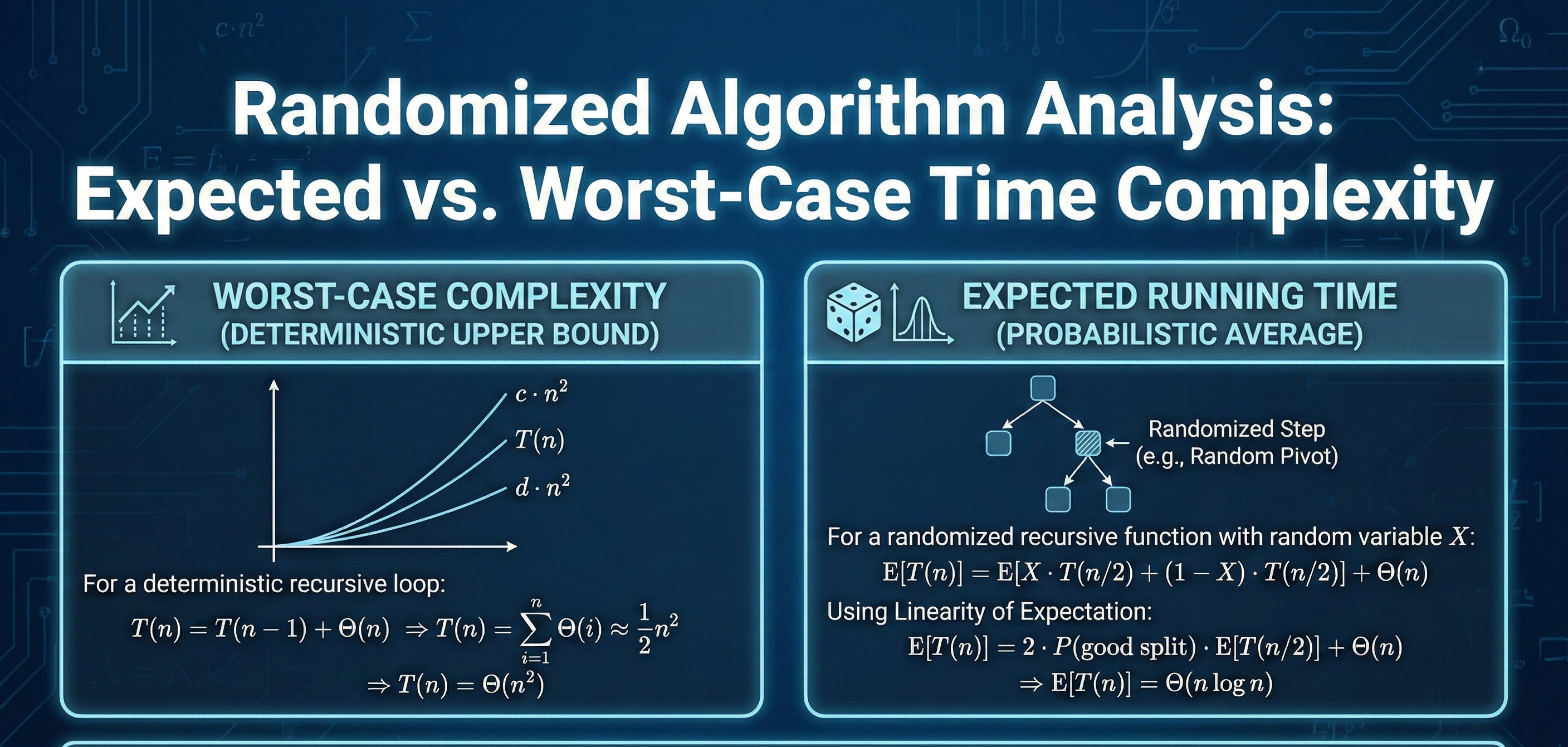
A comprehensive solution set for analyzing the time complexity of randomized algorithms. This download includes step-by-step derivations for Worst-Case and Expected Running Time $E[T(n)]$ using probabilistic analysis, summation approximations, and bounds for recursive functions with random variables.
1. (10 points) Consider the following function: 1 function func1(A, n) 2 s ← 0; 3 k ← Random(n); 4 for i0 ← 1 to k do 5 for i1 ← 1 to k do 6 for i2 ← 1 to ⌊ √ k⌋ do 7 s ← s + A[i0] − A[i1] + A[i2]; 8 end 9 end 10 end 11 return s (a) (2 points) What is the asymptotic worst case running time of func1? (b) (8 points) What is the asymptotic expected running time of func1? Justify your solution with a complete calculation. 2. (10 points) Consider the following function: 1 function func2(A, n) 2 s ← 0; 3 k ← Random(⌊4 log2 (n)⌋); 4 for i ← 1 to 2 k do 5 s ← s + A[i]; 6 end 7 return s (a) (2 points) What is the asymptotic worst case running time of func2? 1 (b) (8 points) What is the asymptotic expected running time of func2? Justify your solution. Hint: 2 4 log2 (n) = (2log2 (n) ) 4 = n 4 . 3. (10 points) Consider the following function: 1 function func3(A, n) 2 s ← 0; 3 k ← Random(n); 4 if k ≤ 7 then 5 for i ← n to ⌊n 5/3 ⌋ do s ← s + i × A[⌈i/n⌉]; 6 else 7 for i ← n to ⌊n log2 (n)⌋ do s ← s + i × A[⌈i/n⌉]; 8 end 9 return s (a) (2 points) What is the asymptotic worst case running time of func3? (b) (8 points) What is the asymptotic expected running time of func3? Justify your solution. 4. (10 points) Consider the following function: 1 function func4(A, n) 2 s ← 0; 3 k ← Random(n); 4 if k ≤ n 2/3 then 5 for i ← n to ⌊n 5/3 ⌋ do s ← s + i × A[⌈i/n⌉]; 6 else 7 for i ← n to ⌊n log2 (n)⌋ do s ← s + i × A[⌈i/n⌉]; 8 end 9 return s (a) (2 points) What is the asymptotic worst case running time of func4? (b) (8 points) What is the asymptotic expected running time of func4? Justify your solution. 5. (15 points) Consider the following recursive function: 1 function func5(A, n) 2 if n ≤ 30 then return A[1]; 3 s ← A[1]; 4 for i0 ← 1 to ⌊n/2⌋ do 5 for i1 ← 1 to ⌊ √ n⌋ do 6 s ← s + A[i0] × A[i1]; 7 end 8 end 9 k1 ← Random(n); 10 k2 ← Random(n); 11 if k1 < 3n/8 then s ← s + func5(A, n − 6); 12 if k2 < 5n/8 then s ← s + func5(A, n − 9); 13 return s 2 (a) (5 points) What is the asymptotic worst case running time of func5? Justify your solution. (b) (10 points) What is the asymptotic expected running time of func5? Justify your solution. 6. (15 points) Consider the following recursive function: 1 function func6(A, n) 2 if n ≤ 40 then return A[1]; 3 s ← A[1]; 4 for i0 ← 1 to ⌊n/2⌋ do 5 for i1 ← 1 to ⌊n/2⌋ do 6 for i2 ← 1 to ⌊n/2⌋ do 7 A[i0] ← A[i0] + A[i0 + i1] − A[i2]; 8 s ← s + A[i0]; 9 end 10 end 11 end 12 k ← Random(n); 13 if k < 3n/4 then s ← s + func6(A, n − 8); 14 return s (a) (5 points) What is the asymptotic worst case running time of func6? Justify your solution. (b) (10 points) What is the asymptotic expected running time of func6? Justify your solution. 7. (15 points) Consider the following recursive function: 1 function func7(A, n) 2 if n ≤ 40 then return A[1]; 3 s ← A[1]; 4 for i ← 1 to n − 7 do 5 A[i] ← A[i] − A[i + 5]; 6 s ← s + A[i]; 7 end 8 k1 ← Random(n); 9 k2 ← Random(n); 10 k3 ← Random(n); 11 if k1 < 2n/7 then s ← s + func7(A, n − 4); 12 if k2 < 2n/7 then s ← s + func7(A, n − 9); 13 if k3 < 2n/7 then s ← s + func7(A, n − 15); 14 return s (a) (5 points) What is the asymptotic worst case running time of func7? Justify your solution. (b) (10 points) What is the asymptotic expected running time of func7? Justify your solution. 8. (15 points) Consider the following recursive function: 3 1 function func8(A, n) 2 if n ≤ 20 then return A[1]; 3 s ← A[1]; 4 for i ← 1 to ⌊n/2⌋ do 5 for j ← 1 to ⌊log2 (n)⌋ do 6 A[i] ← A[i] + A[i + j]; 7 s ← s + A[i] − A[j]; 8 end 9 end 10 k1 ← Random(n); 11 k2 ← Random(n); 12 if k1 < 5n/9 then s ← s + func8(A, n − 8); 13 if k2 < 5n/9 then s ← s + func8(A, n − 13); 14 return s (a) (5 points) What is the asymptotic worst case running time of func8? Justify your solution. (b) (10 points) What is the asymptotic expected running time of func8? Justify your solution. Hint: Pay attention to the sum of the branch probabilities! E
XYZ
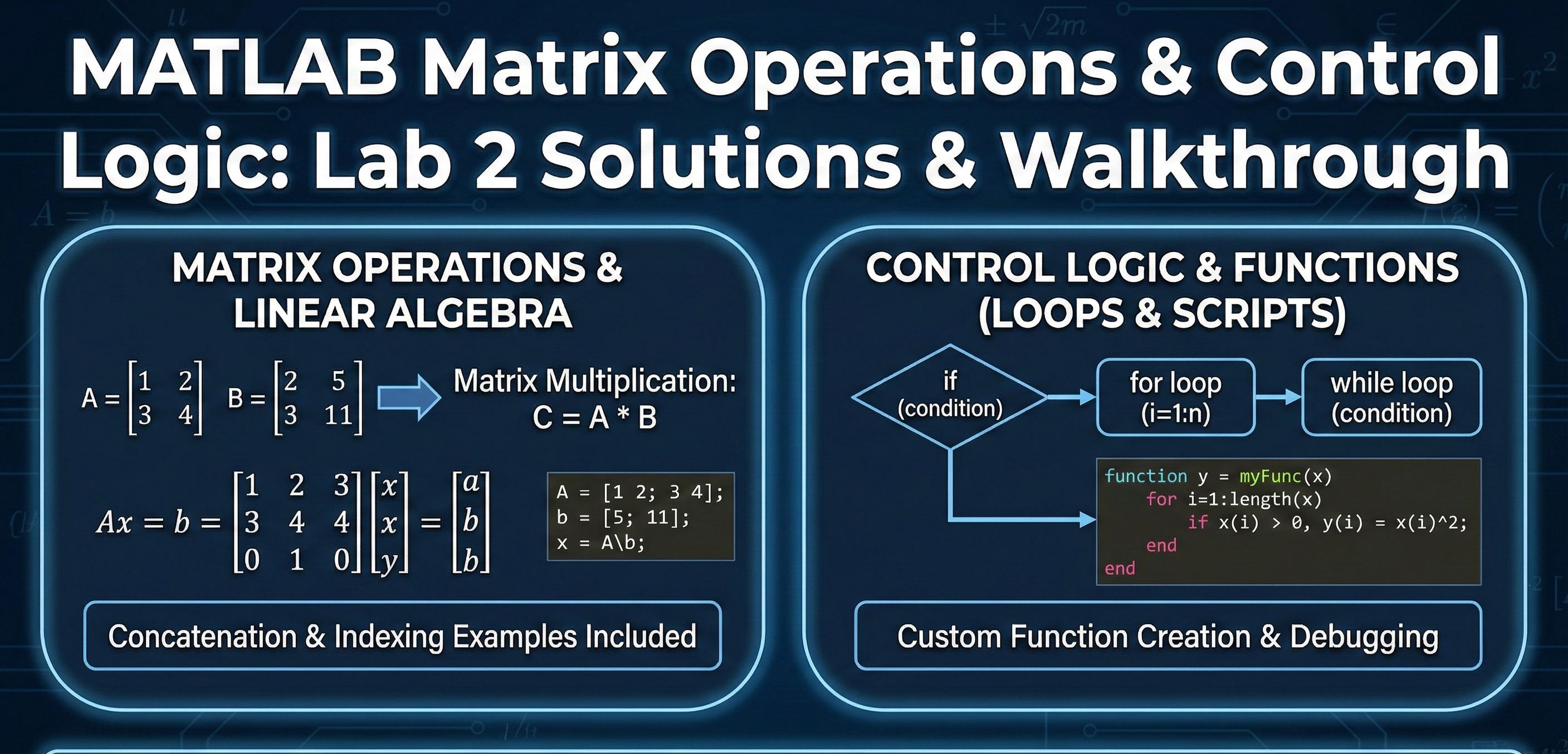
A complete guide to fundamental MATLAB programming. This download includes solutions for matrix manipulation (multiplication, concatenation, indexing) and linear system solving ($Ax=b$), along with a step-by-step walkthrough for implementing control structures (for/while loops) and custom functions.
The objective of this laboratory assignment is to develop proficiency in fundamental MATLAB programming and matrix algebra.The core technical challenge involves three distinct areas:Matrix Manipulation: Users must define, index, and manipulate multi-dimensional arrays, performing operations such as transposition, concatenation, and element-wise arithmetic.Linear Systems: The project requires setting up and solving systems of linear equations of the form $A\mathbf{x} = \mathbf{b}$ using MATLAB's backslash operator to find unknown vector variables.Control Logic: The final phase involves implementing algorithmic logic, specifically utilizing for and while loops to compute geometric series summations and designing a user-defined piecewise function using if-elseif-else conditional statements.
XYZ
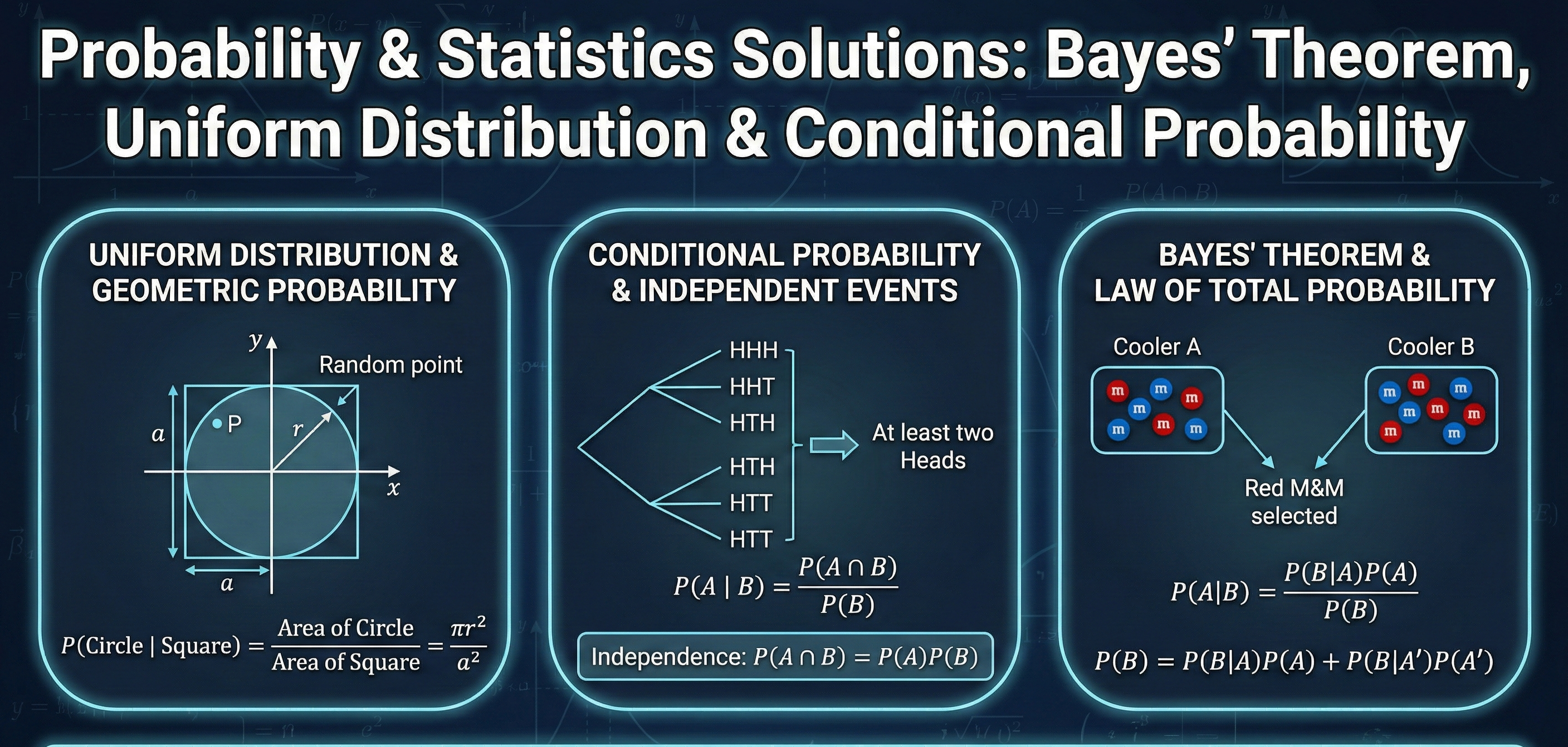
A comprehensive solution set for advanced probability problems. This download covers uniform distribution on geometric regions (Square vs. Circle), conditional probability with independent events (Coin Flips), and complex Bayes' Theorem applications involving the "Cooler" and "M&Ms" scenarios.
Problems: 1. [15 points] Suppose that a point (x, y) is chosen from the square S = [−1, 1] × [−1, 1] using the uniform probability law. Note that since the area of S here is 4, we have P ((x, y) ∈ A) = area(A) 4 for all A ⊂ S. (a) Sketch the regions of the plane corresponding to the events A = {|x| + |y| ≤ 1} B = {|x| 2 + |y| 2 ≤ 1}. (b) Calculate P (B | A). (c) Calculate P (A | B). 2. [10 points] Tom flips two fair coins: a dime and a penny. We will assume that the two coin flips are independent of one another. (a) What is the probability that both coins come up heads? 1 (b) You learn that at least one of the coins has come up heads. What is the probability, conditioned on this information, that both coins came up heads? (c) You learn that the dime has come up heads. What is the probability, conditioned on this information, that both coins came up heads? 3. [15 points] Alice’s cooler contains 13 lemonades and 5 Sprites. Bob’s cooler contains 3 lemonades and 8 Sprites. Unfortunately, the two coolers look identical, making them indistinguishable from the outside. (a) Suppose Bob selects a cooler at random and then chooses a drink at random. What is the probability it is a lemonade? (b) Suppose that the drink he chose was indeed a lemonade. What is the probability he is choosing from his own cooler? (c) Now suppose he pulls out two more drinks, both of which are lemonades. Now what is the probability he is choosing from his own cooler? 4. [10 points] M&Ms come in six colors: brown, yellow, green, blue, red, and orange. Suppose that, in a regular pack of M&Ms, these colors appear with equal probability and according to the uniform law. Mars Inc., which manufactures M&Ms, is running a contest in which one out of every 100,000 packages contain only green M&Ms; if you find such a package, you win a lavish prize. You purchase a pack, and begin taking out M&Ms... (a) Suppose that you pull out 5 M&Ms and they are all green. What is the probability that you are holding a winning package? Note: For the purpose of this problem, you may assume that the package contains an effectively infinite supply of M&Ms so that for a normal package, the probability of a green M&M is 1/6 regardless of how many M&Ms you have already drawn. (b) Suppose you pull out a 6th green M&M. Now, what is the probability you are a winner? (c) What about after a 7th green M&M? Are you excited yet? (d) How many green M&Ms must you pull out to be at least 99% sure you are a winner?
XYZ
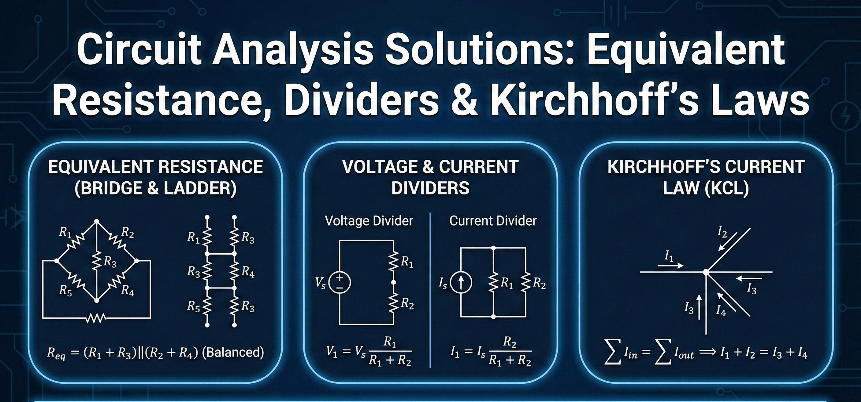
A complete solution set for solving complex resistor networks. This download includes step-by-step calculations for finding equivalent resistance in bridge and ladder circuits, applying Voltage and Current Divider rules, and using Kirchhoff's Current Law (KCL) to solve for unknown branch currents.
Problem 1 (10 Points). Calculate the equivalent resistance of the following circuit. Problem 2 (7 points). Use a current divider to find the current through each resistor. AREN 3040 Circuits for AREN Spring 2026 Problem 3 (8 points). Determine the current through the 2 Ohm resistor assuming the voltage between terminals A and B is 2 V. You can use any method you wish. HOMEWORK 3 Problems 4-7 (20 points). For the following circuits, find the indicated unknowns (marked with question marks) using voltage and current dividers. AREN 3040 Circuits for AREN Spring 2026 Problem 8 (10 points). Find the current I2 in the circuit below. Problem 9 (5 points). Find the equivalent resistance between points A and B.
The Ohio State University
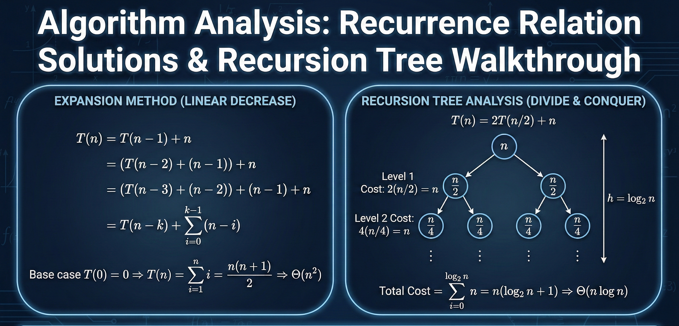
A complete guide to solving Recurrence Relations without the Master Theorem. This download includes detailed solutions for 10 algorithmic problems using the Expansion Method and Recursion Tree Analysis, covering linear decrease, divide-and-conquer, and exponential branching complexity patterns.
1. (Not Graded – Practice Problem) Analyze the running time of the following algorithm: 1 for i ← 8 to ⌊n 3/2 ⌋ do 2 for j ← 40 to i 2 ⌊(log4 i) 2 ⌋ do 3 x ← x + 1; 4 end 5 end (a) Write a formula for the running time T(n). (b) Simplify to get T(n) ∈ Θ(?). 2. (20 points) Analyze the running time of the following algorithm: 1 for i ← 2n to 4n 3 do 2 j ← ⌊√ i⌋; 3 while j > 16 do 4 x ← x + 1; 5 j ← j − 5; 6 end 7 end (a) Write a formula for the running time T(n). (b) Simplify to get T(n) ∈ Θ(?). 1 3. (Not Graded – Practice Problem) Analyze the running time of the following algorithm: 1 for i ← 3n to ⌊n 3/2 ⌋ do 2 for j ← 2n to i do 3 x ← x + (i − j + 1); 4 end 5 end (a) Write a formula for the running time T(n). (b) Simplify to get T(n) ∈ Θ(?). 4. (Not Graded – Practice Problem) Analyze the running time of the following algorithm: 1 for i ← 5 to n 3 do 2 j ← i 2 ; 3 while j > 23 do 4 x ← x + 1; 5 j ← ⌊j/7⌋; 6 end 7 end (a) Write a formula for the running time T(n). (b) Simplify to get T(n) ∈ Θ(?). 5. (20 points) Analyze the running time of the following algorithm: 1 i ← 15; 2 while i ≤ n 3 do 3 for j ← 1 to n 3/i do 4 x ← x + 1; 5 end 6 i ← 7 · i; 7 end (a) Write a formula for the running time T(n). (b) Simplify to get T(n) ∈ Θ(?). 6. (Not Graded – Practice Problem) Analyze the running time of the following algorithm: 1 i ← 5; 2 while i ≤ n 2 do 3 for j ← 1 to ⌊i/2⌋ do 4 x ← x + 1; 5 end 6 i ← 8 · i; 7 end 2 (a) Write a formula for the running time T(n). (b) Simplify to get T(n) ∈ Θ(?). 7. (20 points) Analyze the running time of the following algorithm: 1 i ← 18; 2 while i ≤ n 2.5 do 3 j ← n 2 ; 4 while j > 16 do 5 x ← x + 1; 6 j ← j − ⌈√ n⌉; 7 end 8 i ← 5 · i; 9 end (a) Write a formula for the running time T(n). (b) Simplify to get T(n) ∈ Θ(?). 8. (20 points) Analyze the running time of the following algorithm: 1 i ← n; 2 while i ≥ 15 do 3 j ← 12; 4 while j < 5i do 5 x ← x + 1; 6 j ← j + 8; 7 end 8 i ← ⌊i/3⌋; 9 end (a) Write a formula for the running time T(n). (b) Simplify to get T(n) ∈ Θ(?). 9. (20 points) Analyze the running time of the following algorithm: 1 for i ← 75 to n 2 step 12 do 2 for j ← 6 to 5i do 3 x ← x + 1; 4 end 5 end (a) Write a formula for the running time T(n). (b) Simplify to get T(n) ∈ Θ(?). 3 10. (Not Graded – Practice Problem) Analyze the running time of the following algorithm: 1 i ← n 2 ; 2 while i ≥ 15 do 3 j ← 6; 4 while j < i4 do 5 x ← x + 1; 6 j ← j + i; 7 end 8 i ← ⌊i/5⌋; 9 end (a) Write a formula for the running time T(n). (b) Simplify to get T(n) ∈ Θ(?).
The Ohio State University
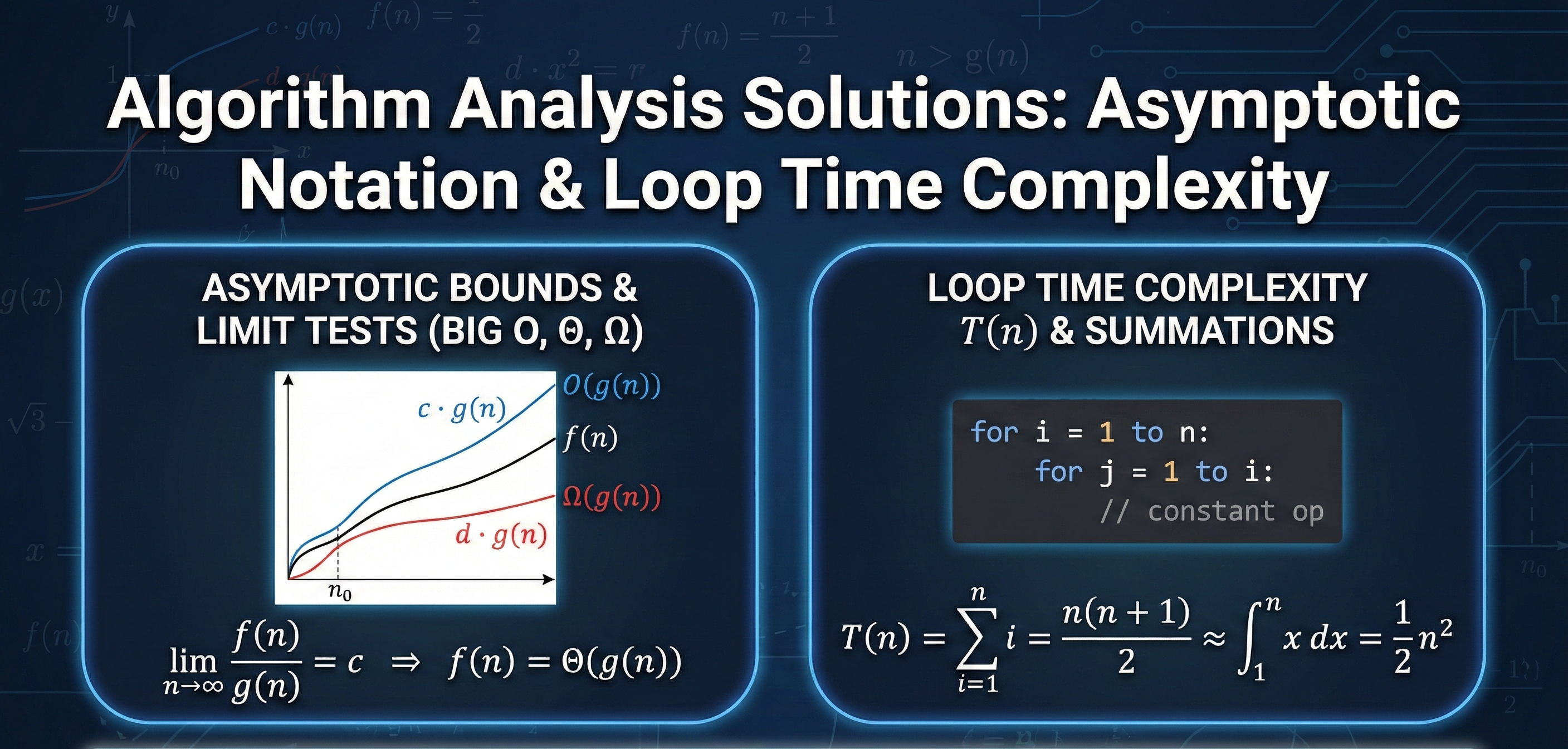
A comprehensive solution set for analyzing algorithm performance. This download includes detailed proofs for asymptotic bounds (Big O, Theta, Omega) using limits and formal definitions, along with step-by-step derivations of time complexity $T(n)$ for nested loops using integral approximation and summation techniques.
1. (8 points) Give an example of a function f(n) such that: • f(n) ∈ O(n 3 ) but f(n) ̸∈ Θ(n 3 ) and f(n) ∈ Ω(n 2 log2 (n)) but f(n) ̸∈ Θ(n 2 log2 (n)). Justify your answer. 2. (8 points) Give an example of a function f(n) such that: • f(n) ∈ O(n 0.5/ log2 (n)) but f(n) ̸∈ Θ(n 0.5/ log2 (n)) and f(n) ∈ Ω((log2 n) 2 ) but f(n) ̸∈ Θ((log2 n) 2 ). Justify your answer. 3. (10 points) Prove that 4 p 7n9 − 12n7 + 5n5 + 3 ∈ Θ(n 4.5 ) using the definition of Θ as functions f(n) such that c1 · n 4.5 ≤ f(n) ≤ c2 · n 4.5 for constants c1, c2 > 0 and all sufficiently large n. Requirements: • Give a rigorous proof that does not simply ignore lower-order terms. • Clearly show how you handle the negative term −12n 7 . • State your values of c1, c2, and n0. 4. (10 points) Prove that 6n 4 log2 (5n 3 + 3n 2 + 2n + 1) ∈ Θ(n 4 log3 (n)) using the definition of Θ. Requirements: • Give a rigorous proof that does not simply ignore lower-order terms. 1 • Use logarithm properties appropriately. • State your values of c1, c2, and n0. 5. (8 points) Let f(n) = 2√ 3 n 2 log4 (n 2 ) and g(n) = 5√ n4 + n3. Using limits, prove that f(n) ∈ Ω(g(n)) but f(n) ̸∈ Θ(g(n)). Requirements: • Compute limn→∞ f(n) g(n) explicitly. • Show all algebraic simplifications. • State what the limit value tells you about the asymptotic relationship. 6. (6 points) Determine the asymptotic bound (in Θ notation) for the following summation: nX2 i=1 i Show your work using the closed-form formula for arithmetic series.
George Mason University
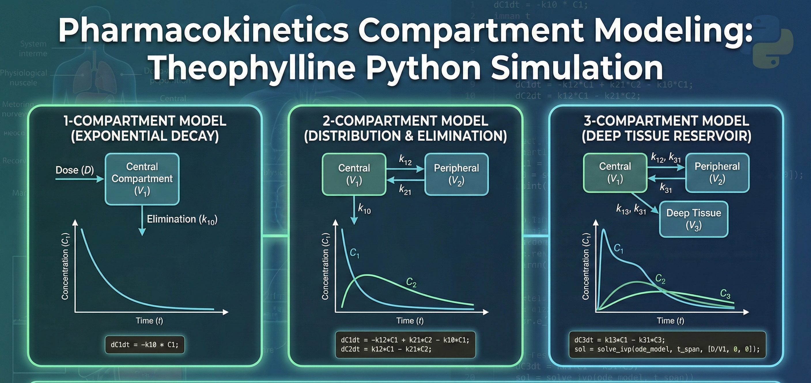
A comprehensive simulation project for analyzing drug distribution (Theophylline) using compartment modeling. This download includes Python scripts for solving 1-compartment, 2-compartment, and 3-compartment differential equations (ODEs) to visualize plasma concentration, elimination phases, and the deep-tissue reservoir effect.
Question 1 (20 pts). A 70 kg patient is administered a single 300 mg oral dose of Theophylline. Assume that absorption and elimination follow first-order kinetics, and the volume of distribution of the drug is the blood plasma only. The absorption rate constant is ka = 1.1 hr-1 , the elimination rate constant is ke = 0.17 hr−1, volume of distribution is Vd=35 L. Assume 100% absorption. Using the following ODE to model the concentration of Theophylline in the plasma: dC(t)/dt = (F ⋅ D_0 ⋅ k_a)/V_d ⋅ e^(-k_a t) - k_e ⋅ C(t) Where D0 is the initial dose and F is the absorption fraction, Solve the ODE numerically in Python to find the concentration-time profile for the drug over 24 hours. Plot the plasma concentration C(t) vs. time and find the peak plasma concentration (C_max) and the time to reach it (T_max). Question 2 (35 pts). You find that the model of Theophylline fails to be validated with experimental data and decide to adjust your assumption that the drug is distributed only through the blood plasma. Now consider that Theophylline distributes between a central compartment (plasma) and a peripheral compartment (tissues). After a 300 mg IV bolus dose, the drug distributes between the compartments with known transfer rates. Elimination rate from central compartment ke = 0.17 hr−1 Transfer rate from central to peripheral k12 = 0.1 hr−1 Transfer rate from peripheral to central k21 = 0.05 hr−1 Volume of distribution in central compartment Vd1 = 35 L Using the following system of ODEs to model the concentrations in the central and peripheral volumes, (dC_1 (t))/dt=-k_12⋅C_1 (t)+k_21⋅C_2 (t)-k_e⋅C_1 (t) (dC_2 (t))/dt=k_12⋅C_1 (t)-k_21⋅C_2 (t) Solve the system numerically to simulate the drug concentrations in both compartments over 24 hours. Analyze and compare the concentration-time profiles for the central and peripheral compartments. Discuss how the drug’s distribution between the two compartments affects the plasma concentration. Question 3 (45 pts). Once again this model of Theophylline fails to be validated with experimental data. You decide now to further adjust your assumption that the drug is being distributed through only the blood plasma and peripheral tissues. Using one of the conditions listed above that can be treated with Theophylline, justify the decision to model Theophylline transport into deep tissues in addition to central and peripheral volumes. Consider Theophylline to now be distributed in three compartments: plasma (central compartment), tissue (peripheral compartment), and deep tissue (slow peripheral compartment), with different transfer rates. After an IV bolus dose of 300 mg, model the distribution dynamics across all three compartments. Elimination rate from central compartment ke = 0.17 hr−1 Transfer rate from central to first peripheral compartment k12 = 0.1 hr−1 Transfer rate from first peripheral to central k21 = 0.05 hr−1 Transfer rate from first peripheral to deep tissue k13 = 0.02 hr−1 Transfer rate from deep tissue to first peripheral k31 = 0.01 hr−1 Volume of distribution in the central compartment Vd1 = 35 L Using the following system of three ODEs for central, peripheral, and deep tissue comparments, (dC_1 (t))/dt=-k_12⋅C_1 (t)+k_21⋅C_2 (t)+k_31⋅C_3 (t)-k_e⋅C_1 (t) (dC_2 (t))/dt=k_12⋅C_1 (t)-k_21⋅C_2 (t)-k_13⋅C_2 (t)+k_31⋅C_3 (t) (dC_3 (t))/dt=k_13⋅C_2 (t)-k_31⋅C_3 (t) where C1(t), C2(t), and C3(t) are the concentrations in the central, first peripheral, and deep tissue compartments. Solve the system numerically to simulate drug concentrations in each compartment over 48 hours. Discuss the impact of the deep tissue compartment on the drug's overall pharmacokinetics. How does the slow transfer into and out of deep tissue affect the drug’s duration of action in the body?
George Mason University
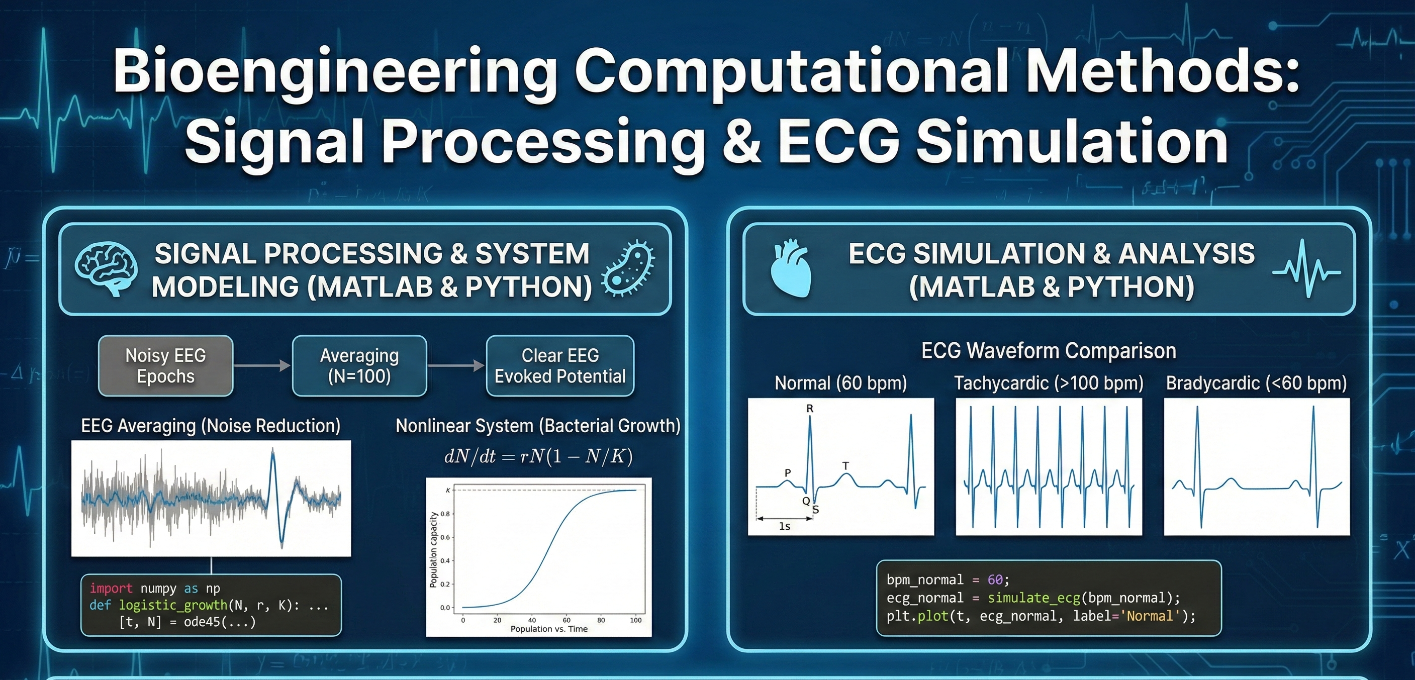
A comprehensive solution set for bioengineering modeling tasks. This download covers the theoretical analysis of EEG signal averaging and nonlinear system verification (bacterial growth), along with complete MATLAB and Python scripts for generating and comparing Normal, Tachycardic, and Bradycardic ECG waveforms.
Question 1 (5 pts). Why is a computer-averaged, EEG-evoked response signal easier to analyze than a raw signal? Question 2 (10 pts). Verify using first principles that the following equation governing bacterial population N in a Petri dish is non-linear: where k and Nmax are fixed parameters. (Hint: Use properties of additivity and proportionality) Question 3 (10 pts). In a left ventricular assist pump, the pressure head P developed across the device is given by the following empirical relationship: where ω is the angular velocity of the pump impeller in units of rad s−1 and QP is the pump flow rate in m3 s−1. If P is in units of Pa (=Nm−2), find the dimensions and units of the coefficients c0, c1 and c2. Question 4 (40 pts). USING MATLAB: Design a system that behaves linearly. Pass through a sine wave with 10 Hz frequency, array length of 1000 pts, and a sampling frequency of 1000 Hz, and plot the input sine wave and the output signal on the same plot. Explain how you can visually determine the system was linear? Question 4 (15 pts). Each equation below represents a straight line. If two lines intersect at one point, then the system of two lines is said to possess a “unique solution.” What type of solution do the following systems of equations (lines) have? Determine by solving the equations using Python. Also plot the equations (lines) to understand the physical significance. In two-dimensional space, how are lines oriented with respect to each other when no solution exists, i.e. the system is inconsistent? What about when there exist infinitely many solutions? Question 5 (20 pts). Access the .m file ECGwaveGen.m from https://www.physionet.org/content/ecgwavegen/1.0.0/#files In MATLAB, plot a normal ECG wave, a tachycardic wave, and a bradycardic wave. Make sure to note the bpm range to be used for each.
George Mason University
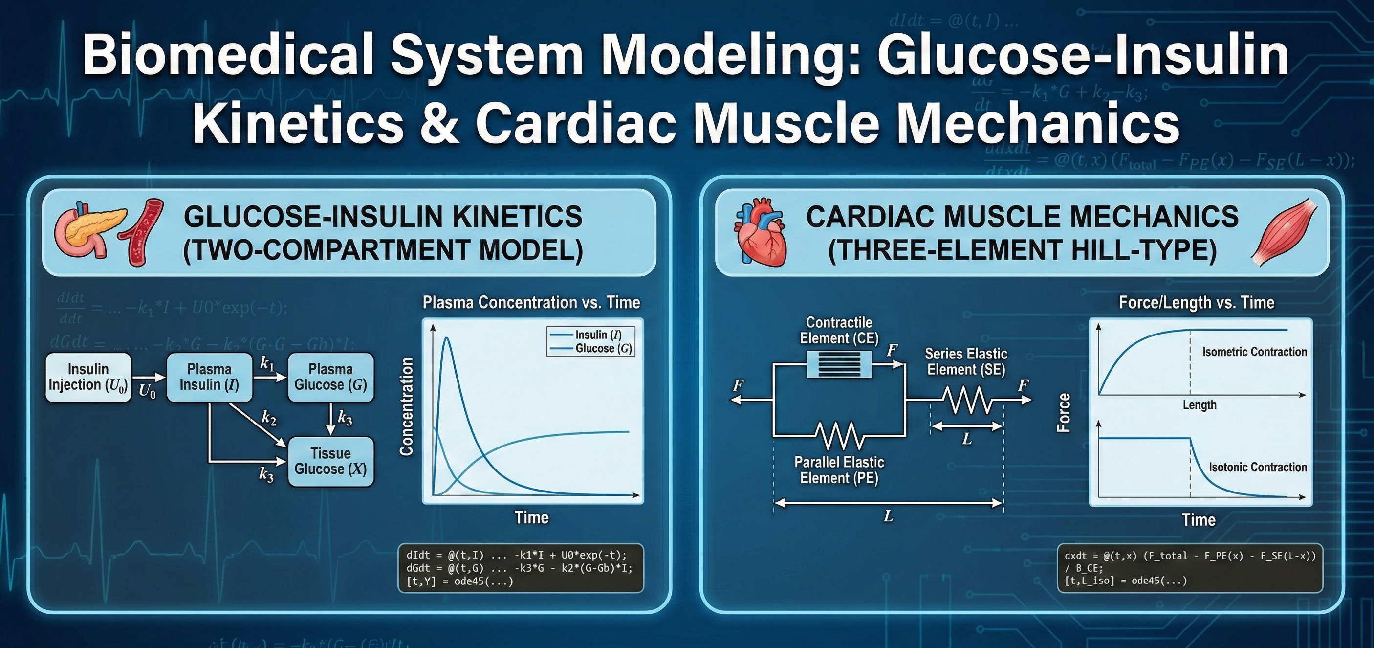
A comprehensive solution set for modeling physiological systems in MATLAB. This download includes a Two-Compartment Glucose-Insulin Model (Berman) to simulate plasma dynamics and a Three-Element Cardiac Muscle Model (Hill-type) to analyze isometric and isotonic contraction mechanics.
Question 1 (20 pts). The passive mechanical behavior of skeletal muscle can be modelled using a simplified lumped parameter representation consisting of a linear spring k1 in series with a parallel linear spring-dashpot combination k2, b, as shown below: One end of the muscle is fixed, and the displacement of the other end is x. If x1 denotes the change in length from rest in spring k1, then the forces in each element are given by: F_1 =k_1 x_1 F_2 =k_2 x_2 F_b =b (dx_2)/dt where F1, F2 and Fb refer to elements k1, k2 and b respectively, and x2 = x − x1. If the length x of the muscle is suddenly stepped and held from 0 to Xm at t = 0, solve the system analytically for the applied force, F. If the applied force on the muscle F is suddenly stepped and held from 0 to Fm at t = 0, find the analytical solution for the change in length, x. Question 2 (30 pts). A simplified two-compartment model of glucose-insulin kinetics in a human subject proposed by Berman et al. is shown below. Ip(t) represents insulin injected intravenously into the blood, I is the concentration of insulin in a remote body compartment, and G is the glucose concentration in the blood plasma. An intravenous dose of insulin is administered as a square-pulse waveform according to: The initial values of I and G at t = 0 are 0 and 10 mM respectively. Solve for I and G using MATLAB over the time interval 0 ≤ t ≤ 60 min. Question 3 (40 pts). A simple three-element model of active cardiac muscle contraction consists of a passive non-linear spring in parallel with a contractile and passive series element, as shown in the diagram. The model structure and equations have been modified from Fung. The total tension T in the muscle is given by the sum of tensions in the parallel and series elements: where Tp and Ts, the tensions in the parallel and series elements respectively, are given by: where α, β are parameters and L0 denotes the resting length of the muscle. For the contractile element, the velocity of its shortening is described by: where a, γ, S0 are muscle parameters and f(t) is the muscle activation function given by with t0 and ti p constants defining activation phase offset and the time to peak isometric contraction respectively. Model parameters for a cardiac papillary muscle specimen are given in the table below: Note that in the relaxed state, the length of the series element Ls is 0. (a) Using Python, solve for and plot the total tension T against time during an isometric contraction in which the muscle is clamped at its resting length L0. (b) Solve for and plot muscle length L against time during an isotonic contraction in which the muscle is allowed to freely contract with no imposed load (i.e. T = 0). Question 4 (10 pts). Consider the left ventricle to be approximated by a spherical shell with inner and outer radii A and B. A uniform pressure is applied to the endocardial (i.e. inner) surface such that the ventricle passively expands to new inner and outer radii of a and b respectively. Assuming that the myocardium is incompressible, find b as a function of a, A, and B.


Get verified answers for your university assignments instantly.

Every homework answer is verified by our AI solver and human experts to ensure A+ grade quality.

No waiting. Search for your coding solution, pay securely, and download the PDF/Source code immediately.

Get unique solutions for helping with homework. Perfect for learning and reference purposes.
Why students globally prefer our solution store

We don't just give answers. Get detailed homework answers with logic explained, ensuring you understand the core concepts.

Looking for coding solutions? Download 100% executable code files (Python, Java, C++) verified by our best Tutors.

No waiting for tutors. Pay for an assignment solution and get the download link immediately via our secure dashboard.

Our expert-verified solutions are designed to help with homework effectively, ensuring you secure top grades in university.

We value your trust. If the Homework solution is incorrect or doesn't match the description, you can claim a full refund.
Get unique content. Every solution in our store is checked against plagiarism tools to ensure originality.