

Home Services Solution Store


Browse our Solution Store for helping with homework. Download complete homework for help solutions, math answers, or pay for an assignment instantly.
XYZ
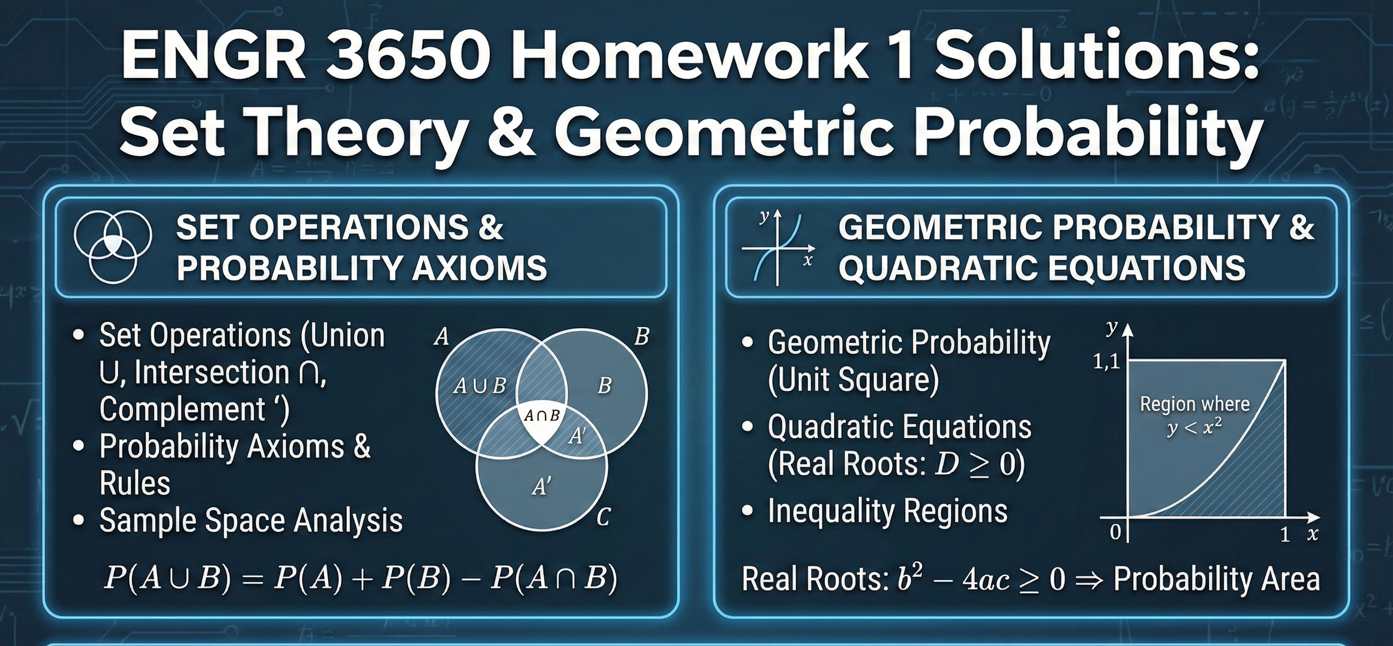
Complete solutions for ENGR 3650 Homework 1. This document covers Set Operations (Union, Intersection, Complement), Probability Axioms, and advanced problems such as calculating the probability of real roots in quadratic equations and solving Geometric Probability inequalities on a unit square.
Problems: 1. [5 points] Suppose our sample space is Ω = {1, 2, 3, 4, 5, 6} and let A = {1, 2, 6}, B = {3, 4}, C = {1, 4, 5}. Find (a) A ∪ B (b) A ∩ B (c) (B ∩ C)c 2. [15 points] The following problems involve applying Kolmogorov’s axioms for probability laws, and properties that follow from Kolmogorov’s axioms. (a) Out of the students in this class, 60% can attend my office hours if I hold them on Monday, 75% can attend them on Friday, and 40% can attend either day. What is the probability that a randomly selected student will not be able to attend my office hours? (b) There is a 50% chance it rains on Saturday, a 60% chance it rains on Sunday, and a 70% chance it rains on Saturday OR Sunday. What is the percent chance it rains on Saturday AND Sunday? (c) Consider the following statements: • the chance it rains on Saturday is 50% 1 • the chance it rains on Sunday is 70% • the chance it rains on both Saturday AND Sunday is 15% Are these statements consistent? In other words, is it possible for all three statements to be true? Justify your answer. (Hint: compute P(A ∪ U) and verify if it satisfies the the axioms.) 3. [5 points] The pieces of candy you are eating come in three flavors: orange, grape, and cherry. When you reach into the bag, the probability you pull out an orange or grape piece is 0.7, while the probability you pull out a grape or cherry piece is 0.9. What is the probability that you pull out an orange or cherry piece? (Hint: Let O, G, and C denote the events that you pull out an orange piece, grape piece, and cherry piece, respectively. You will find the normalization property 1 = P(O) + P(G) + P(C) helpful.) 4. [5 points] Suppose A is a real number chosen on [0, 1] according to the uniform law. Using the value of A, define the quadratic polynomial f(x) = Ax2 + 3x + 4. What is the probability that the roots of f(x) are real? (Hint: The roots of f(x) will be real if and only if the discriminant of the quadratic polynomial is nonnegative.) 5. [15 points] Suppose that a point (x, y) is chosen from the unit square S = [0, 1] × [0, 1] using the uniform probability law — the probability that (x, y) is in a subset A of S is equal to the area of A: P((x, y) ∈ A) = area(A) for all A ⊂ S. (a) What is the probability that x + y < 1/3 ? (b) What is the probability that x + y < 3/2 ? (c) For any real number u, define F(u) := P(x + y ≤ u). Find an expression for F(u) in terms of u. (Hint: for different ranges of u, your expression may change. Just break your answer into a few different cases depending on u.)
The Ohio State University
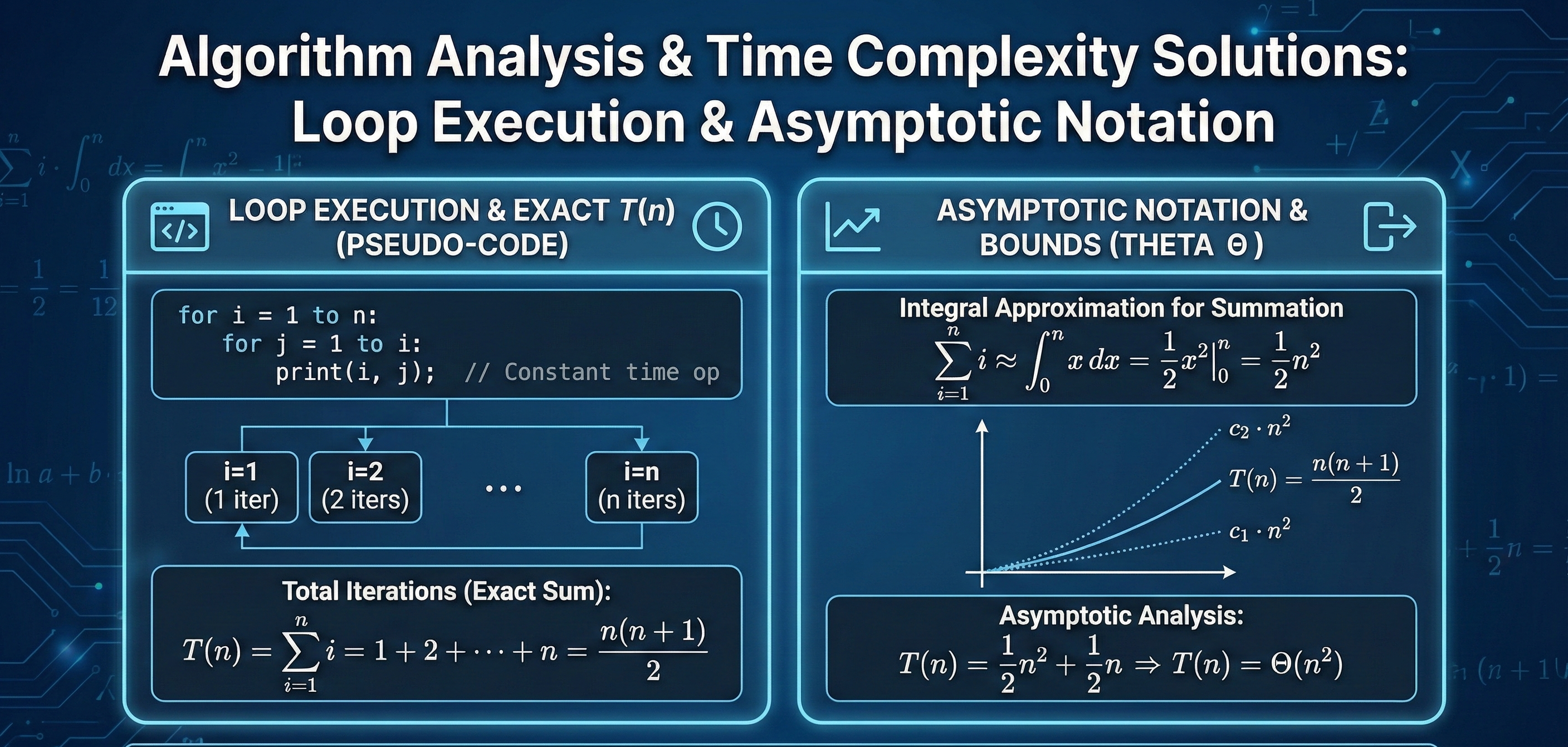
A comprehensive solution set for analyzing the time complexity of various pseudo-code algorithms. This resource derives exact running time formulas $T(n)$ and determines asymptotic bounds (Theta notation) using integral approximations and summation techniques for nested loops and recursive steps.
1. (Not Graded – Practice Problem) Analyze the running time of the following algorithm: 1 for i ← 8 to ⌊n 3/2 ⌋ do 2 for j ← 40 to i 2 ⌊(log4 i) 2 ⌋ do 3 x ← x + 1; 4 end 5 end (a) Write a formula for the running time T(n). (b) Simplify to get T(n) ∈ Θ(?). 2. (20 points) Analyze the running time of the following algorithm: 1 for i ← 2n to 4n 3 do 2 j ← ⌊√ i⌋; 3 while j > 16 do 4 x ← x + 1; 5 j ← j − 5; 6 end 7 end (a) Write a formula for the running time T(n). (b) Simplify to get T(n) ∈ Θ(?). 1 3. (Not Graded – Practice Problem) Analyze the running time of the following algorithm: 1 for i ← 3n to ⌊n 3/2 ⌋ do 2 for j ← 2n to i do 3 x ← x + (i − j + 1); 4 end 5 end (a) Write a formula for the running time T(n). (b) Simplify to get T(n) ∈ Θ(?). 4. (Not Graded – Practice Problem) Analyze the running time of the following algorithm: 1 for i ← 5 to n 3 do 2 j ← i 2 ; 3 while j > 23 do 4 x ← x + 1; 5 j ← ⌊j/7⌋; 6 end 7 end (a) Write a formula for the running time T(n). (b) Simplify to get T(n) ∈ Θ(?). 5. (20 points) Analyze the running time of the following algorithm: 1 i ← 15; 2 while i ≤ n 3 do 3 for j ← 1 to n 3/i do 4 x ← x + 1; 5 end 6 i ← 7 · i; 7 end (a) Write a formula for the running time T(n). (b) Simplify to get T(n) ∈ Θ(?). 6. (Not Graded – Practice Problem) Analyze the running time of the following algorithm: 1 i ← 5; 2 while i ≤ n 2 do 3 for j ← 1 to ⌊i/2⌋ do 4 x ← x + 1; 5 end 6 i ← 8 · i; 7 end 2 (a) Write a formula for the running time T(n). (b) Simplify to get T(n) ∈ Θ(?). 7. (20 points) Analyze the running time of the following algorithm: 1 i ← 18; 2 while i ≤ n 2.5 do 3 j ← n 2 ; 4 while j > 16 do 5 x ← x + 1; 6 j ← j − ⌈√ n⌉; 7 end 8 i ← 5 · i; 9 end (a) Write a formula for the running time T(n). (b) Simplify to get T(n) ∈ Θ(?). 8. (20 points) Analyze the running time of the following algorithm: 1 i ← n; 2 while i ≥ 15 do 3 j ← 12; 4 while j < 5i do 5 x ← x + 1; 6 j ← j + 8; 7 end 8 i ← ⌊i/3⌋; 9 end (a) Write a formula for the running time T(n). (b) Simplify to get T(n) ∈ Θ(?). 9. (20 points) Analyze the running time of the following algorithm: 1 for i ← 75 to n 2 step 12 do 2 for j ← 6 to 5i do 3 x ← x + 1; 4 end 5 end (a) Write a formula for the running time T(n). (b) Simplify to get T(n) ∈ Θ(?). 3 10. (Not Graded – Practice Problem) Analyze the running time of the following algorithm: 1 i ← n 2 ; 2 while i ≥ 15 do 3 j ← 6; 4 while j < i4 do 5 x ← x + 1; 6 j ← j + i; 7 end 8 i ← ⌊i/5⌋; 9 end (a) Write a formula for the running time T(n). (b) Simplify to get T(n) ∈ Θ(?).
George Mason University
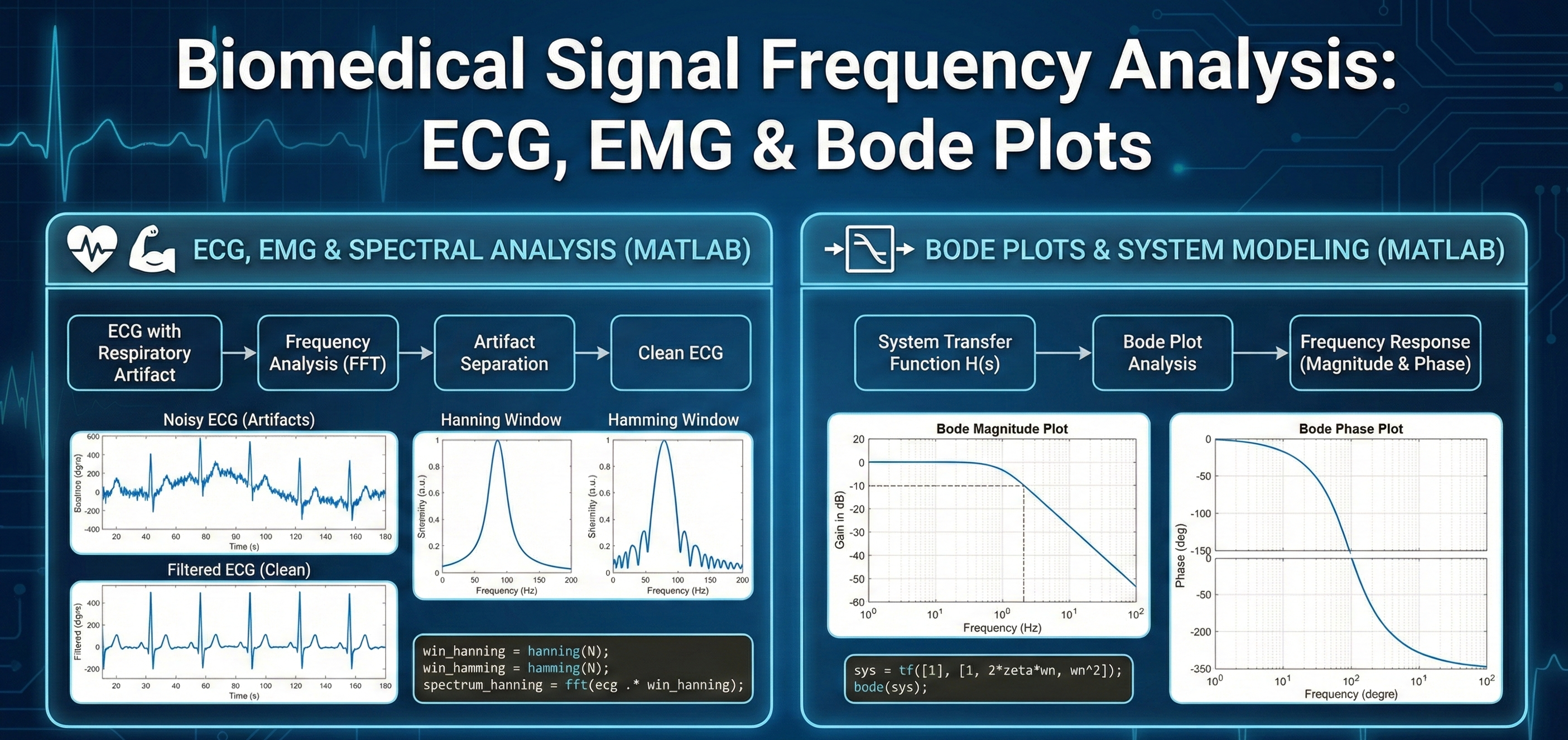
A comprehensive guide to frequency domain techniques in biomedical engineering. This download includes solutions for separating respiratory artifacts from ECG signals, comparing Hanning vs. Hamming windows for spectral analysis, analyzing EMG agonist/antagonist covariance, and modeling system dynamics using Bode plots.
Part 1 (40 pts) Conceptual Questions When recording the ECG using chest leads, the movement due to respiration results in an artifact in the ECG signal. Idealized spectra of the ECG, X1(ω), and the respiration signal, X2(ω), are shown in Fig. 4. Draw the spectrum of the actual measured signal which is a combination of the two. Can they be separated using a filter? Explain what kind of filter can be used to extract the ECG and whether the entire ECG will be extracted. Describe how you could obtain an impulse response estimate of muscle activation from EMG to force data. What assumptions are required for the system to be modeled as LTI (linear time invariant)? If you were to convolve an input spike train (motor neuron firing) with this impulse response, what output would you expect to see? A noisy ECG was filtered three separate times with different filters as shown in figure B. Identify each filter as either a low pass, high pass, band stop, or band pass filter, and match each filter to the correct output. You are analyzing EMG signals using FFT. Compare the Hamming vs Hanning windows: how do they affect spectral leakage and frequency resolution? If you have 2 minutes of EMG sampled at 1000 Hz, what trade-offs arise if you choose 1-s vs 10-s window lengths? Build Hanning and Hamming windows using a half raised cosine function (do not use the built-in hann() and hamming() commands). Run a simple test: compute the FFT of a sinusoid plus noise with both window types and discuss the differences. Use 1000 Hz as the sampling frequency and N = 4000. Select your own frequency and amplitudes for the signal and the noise. Hann (Hanning) window: w_"hann" [n]=0.5(1-cos(2πn/(N-1))) Hamming window: w_"hamming" [n]=0.54-0.46cos(2πn/(N-1)) Part 2 (30 pts) aBP with Embedded Respiration Signal Using the included dataset: abp_with_resp.csv Plot the aBP data. (Must include code and plot here) Research a physiologically typical adult respiration rate (Hz and bpm). Method A (Cross-correlation): Generate a sinusoid at the estimated breathing rate and compute the cross-correlation with the ABP signal. Report the frequency/lag of peak correlation. Method B (FFT): Compute the FFT or Welch spectrum and show that a peak exists at or near the estimated breathing frequency. How close was your estimate to the observed peak? Part 3 (30 pts) Agonist and Antagonist EMG Paired Dataset Use dataset: emg_agonist_antagonist_walking.csv Band-pass filter the raw EMG between 20–450 Hz. This will remove low-frequency _________________ and high-frequency _________________. Calculate the sampling frequency of the given dataset using the diff() command. Compute the power spectral density (PSD) of the filtered EMG using Welch’s method. (Read MATLAB documentation on pwelch). From the PSD, determine the dominant bandwidth (range of frequencies with most EMG power). Based on the Nyquist theorem, select a minimum sampling rate that preserves the identified EMG bandwidth. Compare your chosen rate to the dataset’s given rate. Provide a short paragraph justification of your chosen sampling rate. Select a 10-second segment of agonist and antagonist EMG signals. Calculate the covariance between the two signals: "cov"(x,y)=1/(N-1)∑(x_i-x ˉ)(y_i-y ˉ) Interpret the result (short paragraph, plus covariance value) in terms of whether the two muscles are positively correlated, negatively correlated, or independent. The following is a transfer function with a time delay, which can represent any number of physiological processes. Construct Bode Plots for the following and identify all poles and zeros of the transfer function. G(s)= 100/(s+30) e^(-0.01t)
XYZ
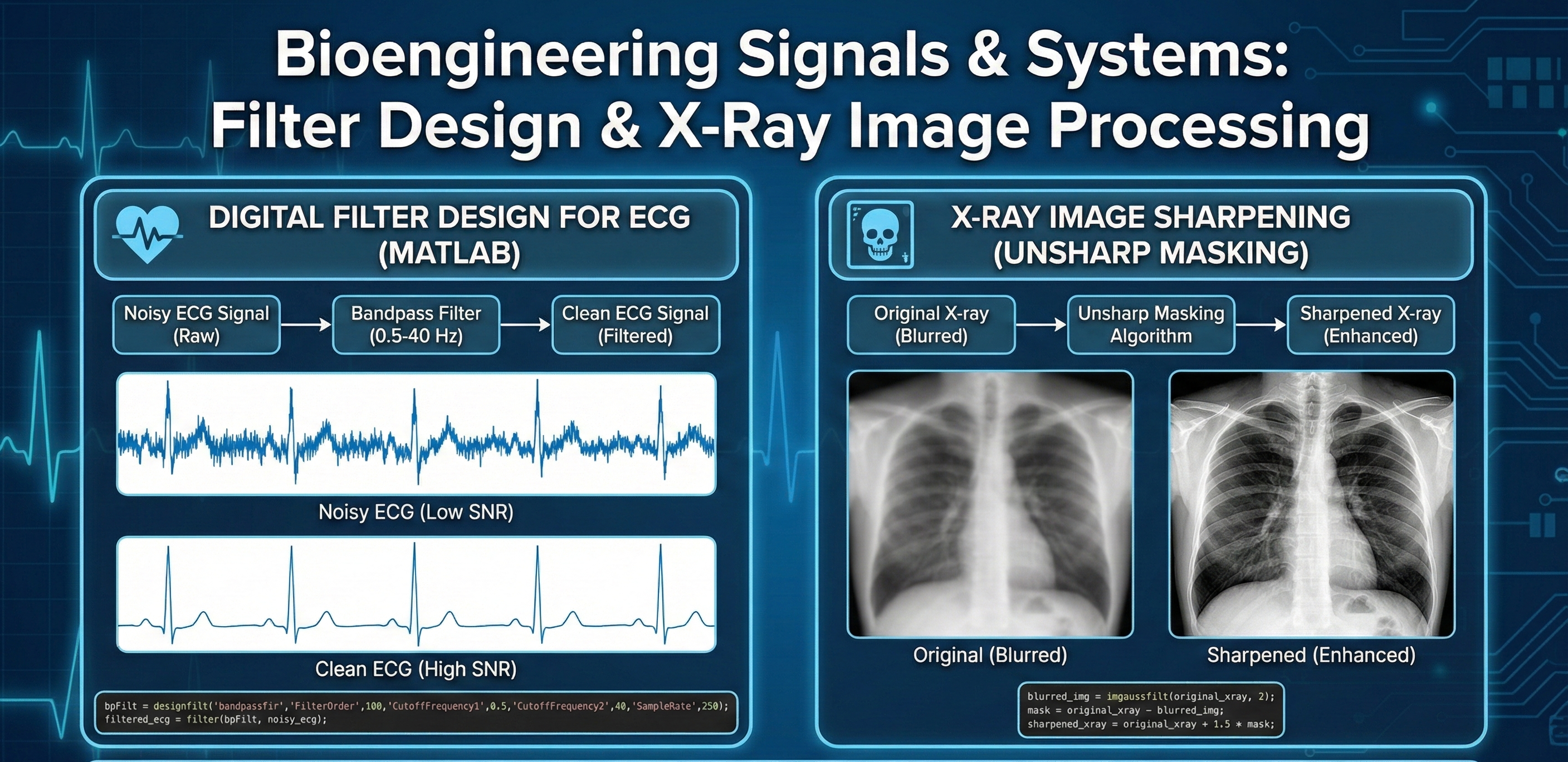
A comprehensive resource for biomedical signal analysis and image enhancement in MATLAB. This download includes theoretical analysis of noise in biosystems (ECG, EEG, MRI), practical code for implementing digital filters (Low-pass, High-pass, Bandpass) to improve ECG Signal-to-Noise Ratio (SNR), and an unsharp masking algorithm for sharpening X-ray images.
Question 1 (15 pts) Describe three biological or biomedical systems/signals that often require filtering (e.g., ECG, EEG, MRI). Identify sources of unwanted components (noise, artifacts, or irrelevant frequencies) in each case, and explain why filtering is necessary Question 2 (15 pts) Find a dataset of a 1D biosignal. Find a dataset of a 2D biosignal. Describe each with regards to what it is depicting, what noise is present, and what kind of filtering each would require. Load datasets into MATLAB and show plots. Question 4 (20 pts) Develop a moving average filter for the ECG signal included with the project and the 1D dataset found in Question 2. Describe the pseudocode below, then implement in MATLAB and show the “before” and “after” graphs. Question 5 (10 pts) Introduce random noise to both of your biosignals (using MATLAB). Show the “before” and “after”. Question 6 (20 pts) Now run a low pass, high pass, and bandpass filter on the signals. Describe your findings regarding the random noise and the “before” and “after” of each signal. What do the filters tell you about the introduced noise? Question 7 (20 pts) Implement the code below with the image provided. Describe what the code is doing and how it impacts the image provided. Show all output.
XYZ
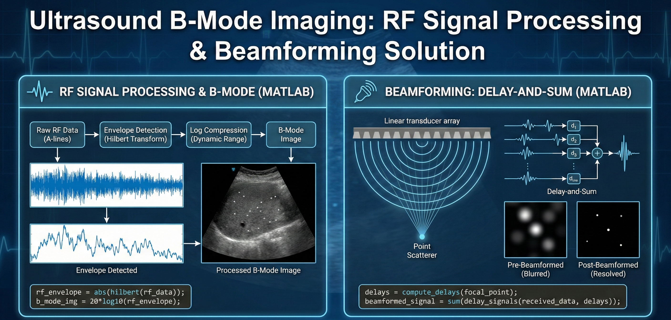
A detailed solution for processing raw ultrasound RF data into clear B-mode images using MATLAB. This download covers envelope detection (Hilbert transform), log compression, and the implementation of Delay-and-Sum beamforming to resolve point scatterers and remove image blurring.
1. Signal processing for B-mode image A linear ultrasound array with 128 active elements was used to acquire image data (US_prebeamformed.mat) from a tissue-mimicking medium with several nylon strings acting as point scatterers. The image is 38.4 mm long and 57.75 mm long. a. We discussed that envelop detection and log compression improves visualization of image. A pseudo-code for this as is follows: i. Compute the magnitude of the Hilbert transform (this gives envelope) to obtain the envelope. ii. Divide the envelope image with its maximum value – referred to as normalization. iii. Compute the log-base-10 of the normalized envelope and multiply by 20. Use the imagesc function, “figure, imagesc([0 38.4],[0 57.75],image_variable)”, to display the raw ultrasound data, envelope image, and log compressed image. Note that the dynamic range of the log-compressed image may have to be adjusted as follows: “figure, imagesc([0 38.4],[0 57.75],image_variable,[-40 0])”. Describe the differences in each image. Use the colorbar function to see the range of image-intensity values. What are the maximum and minimum values of the log-compressed image? Do you see the point scatterers? If not, explain why not? b. Use the included beamformDAQ function, “bmRF = beamformDAQ(RF, 32);”, to apply delay-and-sum beamforming to the raw ultrasound data with a moving aperture of 32 elements. Compute the envelope and log-compressed images of the beamformed data. Compare the log-compressed-envelope image of the beamformed data to that from the raw (not beamformed) data and describe the difference. Why are the point targets visible?
XYZ
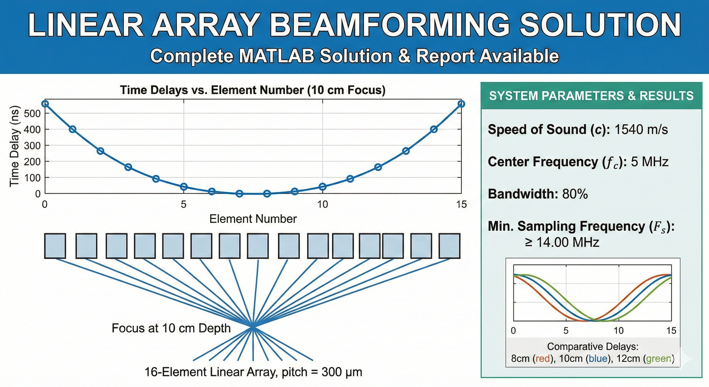
A complete technical guide for designing a Linear Phased Array Beamforming system. This download includes a solution report detailing the calculation of geometric time delays and sampling frequencies for a 16-element ultrasound array, paired with a MATLAB walkthrough for simulating beam focusing at multiple depths.
Linear Array Transmit Beamforming and Sampling RequirementsContext:You are designing the transmit beamformer for a linear ultrasound array. The system needs to focus energy at specific depths along the central axis of the array. You are tasked with calculating the required time delays for the elements and determining the necessary sampling parameters for the system.System Parameters:Array Type: Linear ArrayNumber of Elements ($N$): 16Element Pitch ($d$): $300 \mu m$Speed of Sound ($c$): $1540$ m/sCenter Frequency ($f_c$): 5 MHzFractional Bandwidth: 80%Tasks:Delay Calculation (10 cm Focus):Calculate the transmit time delays required to focus the beam at a depth of 10 cm on the array's central axis ($x = 0$).Assume the delays are calculated relative to the array center.Ensure all delays are positive values (the element closest to the focal point should have the maximum delay, or conversely, the reference time is set such that the first firing element has $t=0$).Plot the Time Delay (ns) vs. Element Number.Effect of Focal Depth:Repeat the delay calculation for focal depths of 8 cm (shallower) and 12 cm (deeper).Generate a single comparative plot showing the delay profiles for all three depths (8 cm, 10 cm, and 12 cm) on the same axes.Observe how the curvature of the delay profile changes as the focal depth increases.Sampling Frequency Requirements:To accurately synthesize these delays digitally, the system requires a sufficient sampling clock.Calculate the upper cutoff frequency ($f_{max}$) of the transducer based on the center frequency and bandwidth.Determine the minimum sampling frequency ($F_s$) required to satisfy the Nyquist criterion for the signal band.
George Mason University
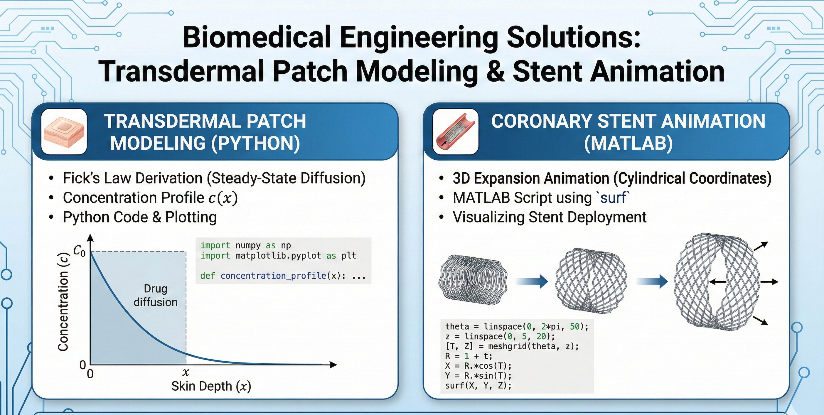
A complete solution guide for biomedical modeling tasks. This download includes the mathematical derivation and Python simulation for steady-state drug delivery via transdermal patches (Fick's Law), along with a MATLAB script for animating the expansion of a coronary stent.
Question 1 (50 pts). A transdermal patch is placed on the arm of a patient to deliver a specific dose of medication through the skin. The equation governing the concentration c of the drug is ∂c/∂t=D (∂^2 c)/(∂x^2 )- k_up c where x is the depth through the skin, D is the diffusion coefficient and kup is the rate of uptake of the drug into the bloodstream. Find the steady-state concentration as a function of x given the boundary conditions c = C0 at x = 0 (skin surface) and c = 0 at x = dc (critical depth). D, kup, C0 and dc are fixed parameters. Fentanyl patches are typically designed to deliver a steady dose over an extended period, and the drug concentration can vary based on skin depth. Taking the diffusion coefficient D as 1×10⁻⁹ cm2/s, and starting concentration at the surface as 5 mg/cm3, model the drug concentration over skin depth in Python. Take 0.2 cm as critical depth, and select appropriate skin depth intervals. Produce a concentration profile and mark skin depth on the plot where drug concentration is half the initial concentration. For drug A with a critical depth of 0.3 cm, (where the drug reaches a concentration of zero), and a diffusion coefficient of 0.8 x 10⁻⁹ cm2/s, determine C0 using the solution to part a. Assume the transdermal patch is designed to deliver 5 mg of the drug over 24 hours through an area of 10 cm². Suggest dimensions for the transdermal patch if the patch is made of a gel with an absorbency of 2 mg/cm3 Question 2 (50 pts). Create an animation in MATLAB of a coronary stent expanding from an initial radius of 1 cm to 3 cm. Model the stent as a cylinder with initial length of 10 cm. Submit both the code and a screen recording of your animation with your homework.
XYZ
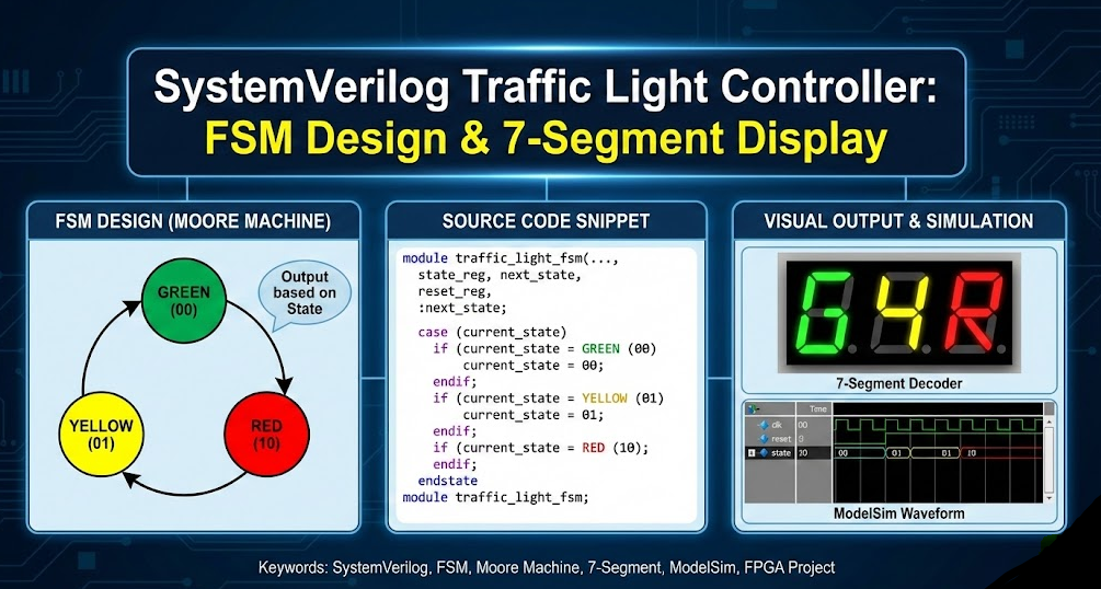
A complete SystemVerilog project for a Traffic Light Controller using a Moore Finite State Machine (FSM). This download includes the source code for cycling through Green, Yellow, and Red states , a 7-segment decoder for visual output , and a ModelSim testbench to verify state transitions and timing .
The objective of this project is to design and verify a digital control system for an automated traffic light. Real-world traffic management relies on precise timing and clear visual feedback to maintain safety. The specific technical challenge is to implement a Finite State Machine (FSM) using SystemVerilog that automatically cycles through a fixed sequence of states: Green (G), Yellow (Y), and Red (R). The system must meet the following requirements: State Control: The controller must transition states (G → Y → R → G) on every clock cycle when the reset is low ("0") and immediately return to the default Green state when the reset is high ("1"). Visual Output: The design must include a 7-segment decoder that translates the internal 2-bit binary state codes (00, 01, 10) into the corresponding 7-bit binary patterns required to display the characters 'G', 'Y', and 'R' on a common 7-segment display. Verification: The functionality of both the FSM and the decoder must be verified through waveform analysis in ModelSim to ensure glitch-free transitions and accurate character representation.
XYZ
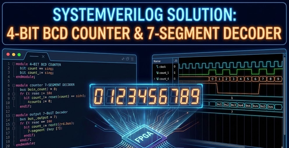
A complete design guide for a 4-Bit BCD Counter with 7-Segment Display output. This download includes a technical report and walkthrough covering the SystemVerilog implementation of sequential counting logic (Modulo-10), combinational decoding, and testbench verification with waveform analysis.
The objective of this project is to design and simulate a synchronous digital system using SystemVerilog that functions as a 4-Bit BCD (Binary Coded Decimal) Counter. The core technical challenge involves implementing specific Modulo-10 logic to restrict the standard 4-bit binary counting range (0–15) to a decade sequence (0–9), ensuring the system correctly resets to zero upon reaching nine. Additionally, the system requires a combinational decoder module to translate the 4-bit binary output into active-high 7-bit control signals suitable for driving a 7-segment display. The final design must be verified through a ModelSim testbench to confirm correct timing, rollover logic, and display mapping.


Get verified answers for your university assignments instantly.

Every homework answer is verified by our AI solver and human experts to ensure A+ grade quality.

No waiting. Search for your coding solution, pay securely, and download the PDF/Source code immediately.

Get unique solutions for helping with homework. Perfect for learning and reference purposes.
Why students globally prefer our solution store

We don't just give answers. Get detailed homework answers with logic explained, ensuring you understand the core concepts.

Looking for coding solutions? Download 100% executable code files (Python, Java, C++) verified by our best Tutors.

No waiting for tutors. Pay for an assignment solution and get the download link immediately via our secure dashboard.

Our expert-verified solutions are designed to help with homework effectively, ensuring you secure top grades in university.

We value your trust. If the Homework solution is incorrect or doesn't match the description, you can claim a full refund.
Get unique content. Every solution in our store is checked against plagiarism tools to ensure originality.