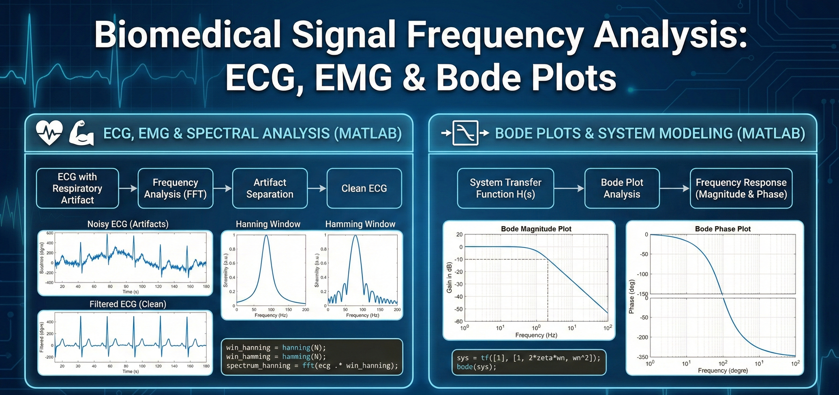
A comprehensive guide to frequency domain techniques in biomedical engineering. This download includes solutions for separating respiratory artifacts from ECG signals, comparing Hanning vs. Hamming windows for spectral analysis, analyzing EMG agonist/antagonist covariance, and modeling system dynamics using Bode plots.
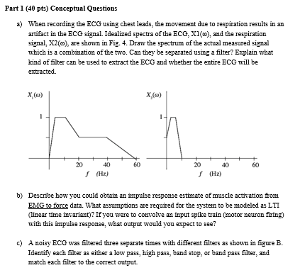
Part 1 (40 pts) Conceptual Questions
When recording the ECG using chest leads, the movement due to respiration results in an artifact in the ECG signal. Idealized spectra of the ECG, X1(ω), and the respiration signal, X2(ω), are shown in Fig. 4. Draw the spectrum of the actual measured signal which is a combination of the two. Can they be separated using a filter? Explain what kind of filter can be used to extract the ECG and whether the entire ECG will be extracted.
Describe how you could obtain an impulse response estimate of muscle activation from EMG to force data. What assumptions are required for the system to be modeled as LTI (linear time invariant)? If you were to convolve an input spike train (motor neuron firing) with this impulse response, what output would you expect to see?
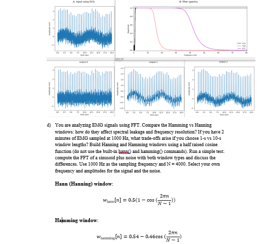
A noisy ECG was filtered three separate times with different filters as shown in figure B. Identify each filter as either a low pass, high pass, band stop, or band pass filter, and match each filter to the correct output.
You are analyzing EMG signals using FFT. Compare the Hamming vs Hanning windows: how do they affect spectral leakage and frequency resolution? If you have 2 minutes of EMG sampled at 1000 Hz, what trade-offs arise if you choose 1-s vs 10-s window lengths? Build Hanning and Hamming windows using a half raised cosine function (do not use the built-in hann() and hamming() commands). Run a simple test: compute the FFT of a sinusoid plus noise with both window types and discuss the differences. Use 1000 Hz as the sampling frequency and N = 4000. Select your own frequency and amplitudes for the signal and the noise.
Hann (Hanning) window:
w_"hann" [n]=0.5(1-cos(2πn/(N-1)))
Hamming window:
w_"hamming" [n]=0.54-0.46cos(2πn/(N-1))
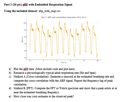
Part 2 (30 pts) aBP with Embedded Respiration Signal
Using the included dataset: abp_with_resp.csv
Plot the aBP data. (Must include code and plot here)
Research a physiologically typical adult respiration rate (Hz and bpm).
Method A (Cross-correlation): Generate a sinusoid at the estimated breathing rate and compute the cross-correlation with the ABP signal. Report the frequency/lag of peak correlation.
Method B (FFT): Compute the FFT or Welch spectrum and show that a peak exists at or near the estimated breathing frequency.
How close was your estimate to the observed peak?
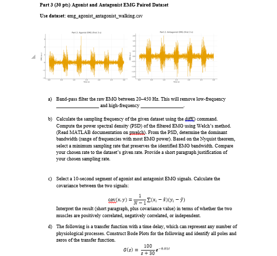
Part 3 (30 pts) Agonist and Antagonist EMG Paired Dataset
Use dataset: emg_agonist_antagonist_walking.csv
Band-pass filter the raw EMG between 20–450 Hz. This will remove low-frequency _________________ and high-frequency _________________.
Calculate the sampling frequency of the given dataset using the diff() command. Compute the power spectral density (PSD) of the filtered EMG using Welch’s method. (Read MATLAB documentation on pwelch). From the PSD, determine the dominant bandwidth (range of frequencies with most EMG power). Based on the Nyquist theorem, select a minimum sampling rate that preserves the identified EMG bandwidth. Compare your chosen rate to the dataset’s given rate. Provide a short paragraph justification of your chosen sampling rate.
Select a 10-second segment of agonist and antagonist EMG signals. Calculate the covariance between the two signals:
"cov"(x,y)=1/(N-1)∑(x_i-x ˉ)(y_i-y ˉ)
Interpret the result (short paragraph, plus covariance value) in terms of whether the two muscles are positively correlated, negatively correlated, or independent.
The following is a transfer function with a time delay, which can represent any number of physiological processes. Construct Bode Plots for the following and identify all poles and zeros of the transfer function.
G(s)= 100/(s+30) e^(-0.01t)